Diagrams with LaTeX – easier than you might think

I’ve written before about the power of literate programming, using to create reports when code runs.  It’s fairly simple to combine this with the graphical drawing packages to create impressive graphs and figures on the fly.  A lot of academics I’ve spoken to have shied away from using for drawing, despite being very proficient with the textual layout.  Similarly, a lot of students on the OU Mathematics degree write up all of their assignments in but drop in hand drawn graphs and diagrams.  Just like anything else in , once you get your head around how it works, it’s actually not that difficult to create very complex structures.

One of the best tools I’ve discovered recently is ShareLatex.com, the equivalent of jsfiddle – very easy for playing around with diagrams and seeing what effect changes will have without having to recompile whole documents and also very easy to share with colleagues when you need a hand.  You need to register to use it and you can create pdf versions easily – fantastic when you don’t have everything you need installed locally but need an updated figure straight away. If you’re using then bookmark that site!  All the code below is available on my GitHub.

If you don’t have a copy of the Graphics Companion¹, which explains everything in detail, like any other programming language, the resources are all available online if you know where to look.  However, I’ll start with a quick example of a few images² and then you can search for the rest :).

Right now, I can imagine that everyone doing the modelling exercise for this year’s MST210 is hoping that I’ll use that problem as an example.  Sorry to disappoint but I won’t do your work for you.  However, all the methods you’ll need are in this post.  Let’s look at exercise 29 from unit 3³.  Neither the question nor the answer to this problem has a diagram, and since I’m not going to solve the problem here (the answer is in the book!⁴) it’s a nice example.

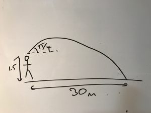
A stone is thrown from a height of 1.5m above horizontal ground at and angle of above the horizontal and lands at a distance of 30m from the point it was thrown.  Estimate the speed with which it was thrown.

One of the first things you’d do is scribble a diagram like this:

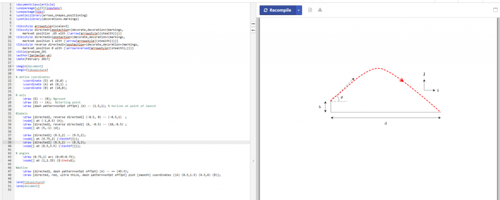
So how to begin drawing this in ?  Well, the first thing you’d do to solve the problem is to start with the axes, so let’s draw some simple lines. I’ve used a package called tikz which is my go to for most diagrams.  Declare it in the standard way and define a picture block with \begin{tikzpicture}.  Using the origin as a starting point we can draw a horizontal line and a vertical line.  I’ve used cm units here as standard.  You should get this:

We’re probably going to use the origin and the start point and end point a few times, so we can define coordinates (O, A and B) and replace these in our lines. For clarity, I’ve also separated out the \draw commands from coordinates.  Now let’s add a dashed line showing the initial direction:

\draw [dash pattern=on5pt off3pt] (A) -- ++ (45:2);

This looks a little complex so I’ll break it down.  We are using the draw command again, but are adding a parameter in the square brackets.  This should be familiar to you.  I’ve overridden the dash default to have an alternating 5pt on, 3pt off pattern.  The (A) is our starting coordinate.  Instead of specifying an end coordinate, I’ve stated an angle of 45 degrees (from horizontal) with a length of 2cm.  Note that this uses the colon rather than a comma.  Rather that the double dash to specify a line from a to b, the angle syntax is drawn as if it originates from the origin.  Here, we’re starting at A so we need to tell tikz that we want this line relative to A and not O: this is achieved with the ++.  Putting that all together gives us:

Let’s add a horizontal line and the angle.  A short dashed line parallel to the x-axis can be defined, but we don’t want it full length so let’s make it length 1.5 so it sits neatly below our initial velocity line.  Now, we want to draw an arc from this new line to show using \draw arc.  An arc needs a starting point, the angles that contain the arc, and a radius.  Since we’re starting from the horizontal this is nice and easy.  Our starting point is (0.75,1) and we want an arc from 0 to 45 degrees.  Since we are parallel with the origin, our radius is simply our x coordinate again (0.75).  Finally we want to label our angle so we define a node just outside of our arc and put a in it.

Now we want to add our motion.  This is another draw command:

\draw [red, ultra thick, dash pattern=on5pt off3pt] plot [smooth] coordinates {(0,1) (0.5,1.5) (4.5,4) (10,0)};

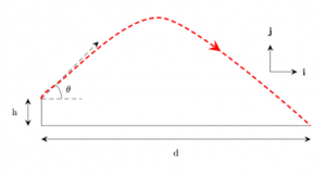
This time, we add to the dash by making the line ultra thick and colouring it red.  The plot [smooth] parameter will draw a smooth curve through the points we specify.  Since we know this is a parabola, we can use A and B as our start and end coordinates⁵ and just before halfway there will be an apex.  Since the drawing is not to scale, you might need a bit of trial and error to get the image to look right.  Here I’ve used a point close to the start to ensure the trajectory stays on the 45 degree angle and then played around with the y-coordinate until I found something that worked.

Finally, let’s add some labels and arrows. We can add labels using the node command as we did to label the angle.  For height and distance we can add further lines offset by 0.5 from the height and distance⁶.  We can also define some arrows to add to our lines.  For this, we add a few extra options to tikz.

I’ve set the arrowstyle to be scale 2 so the arrows are bigger – this is just a personal choice.  I then define three decorations.  Here’s the first:

\tikzstyle directed=[postaction={decorate,decoration={markings,
mark=at position .65 with {\arrow[arrowstyle]{stealth}}}}]

This defines a parameter style called ‘directed’ to add a decoration after drawing the object (the line in this case) putting a mark 65% along the line with an arrow of the style we’ve previously defined.  The other two styles put the arrows at the beginning and end of the line respectively.  Multiple styles can be added to each line so the height label is defined as:

\draw [directed2, reverse directed2] (-0.5, 0) -- (-0.5,1)  ;
\node[] at (-1,0.5) {h};

Adding our i and j vectors and the final code and diagram looks like this:

And there’s the final diagram.  If you want to grab the code for this and have a try yourself, I’ve made my ShareLatex.com project publicly visible. Once you’ve done one, you’ll see how easy it is to create your own diagrams quickly.  There are a whole host of specialist packages out there depending on what sort of diagram you need to draw.  Tikz has a lot of examples, or failing that try googling “latex draw [subject]”.  I’d recommend the Graphics Companion as it does explain all the commands from first principles if you really want to get into the guts of it.  Finally, the stackoverflow LaTex forum is a fantastic place for questions and answers.

Remember that some of the commands are absolute and others reference the origin by default.  With a little planning (perhaps a sketch on some graph paper) you can make life easy for yourself.

Drawing diagrams can make your presentations neater and once you’ve done a few, you’ll see how easy they are.